Conclusion

This is the conclusion of a 3 part series analyzing a betting game. If you'd like to jump to another part here are direct links:

• Intro Page
• Part 1 - A Simpler Problem
• Part 2 - Analysis and Simulations
• Part 3 - Mathematical Restructuring
• Conclusion (You are here)

Differences between Expected Value and Most Probable Value

Throughout this series I kept emphasizing the difference between the expected value of a situation and the most probable value in a situation. As seen, these values can be quite different from each other and have a big impact on how to analyze a situation.

Expected value should be considered when the game will be repeated (many times), while the most probable value makes more sense to consider when given one shot at a game.

In this game there are 2 parameters: the bias of the coin and the number of rounds you get to play. It is worth pointing out that playing multiple games is very different than playing a game with more rounds - your knowledge of the bias of the flipped coin resets between games as the dealer chooses the coin again.

We can show the resulting EV in a heat map over the space of coin biases and rounds of flips, as in the following figure:

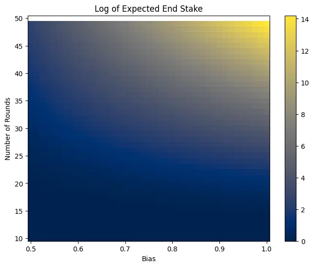
Note that this is graphing the $log_{10}(S)$, so even a value of $2$ signifies a 10,000% return.

We can also simulate the flips to test the distribution of values that we obtain. We will consider a more modest example where $p=0.6$ and $r=20$. For these parameters the expected value is $1.317$ while the most probable return is $0.869$. Here is a histogram showing the results from $10,000$ simulations:

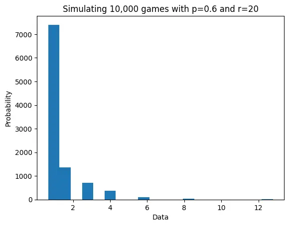
Even though you lose money a little over 50% of the time, your earnings over all trials still average out to around 1.30 per game. The key is that, because of how the Kelly Criterion dictates betting, you will lose small but win big.

If you are only able to play the game once the variance can be extremely high, but if you are able to play the game over and over with re-invested earning the winnings will be huge, in this case approaching $1.3^1000.

For a different example, say the bias in the coins is 0.51, making the coins nearly indistinguishable. Each coin is played for 50 rounds. Here is the graph for this scenario:

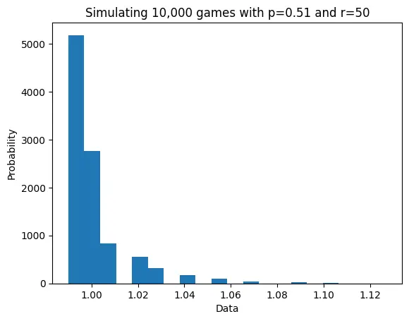
While the game now loses money around $2/3^{rd}$s of the time, and the expected earnings per game are just $1.0002$, over $10,000$ rounds with the stake reinvested each time the game is expected to earn $7.098$, though the variance is high. In this simulation the earnings were $2.531$.

In general the expected value that you can earn after playing $n$ games while reinvesting winnings is $\operatorname {E} [S]^n$ where $\operatorname {E} [S]$ is the expected value of the stake after one game¹. Clearly the expected value dominates and remains more important than the median-probability value in the long run.

Wrap Up

Code for calculating and simulating is in this repo on my GitHub.

This turned out way longer than I initially intended². I planned to use this as a small project that I could do in a week, but I've now been working on it for the better part of a month. On one hand I'm glad that this problem was interesting enough to force me to keep going deeper and get more out of it, but I'm also excited to move onto other things.

Writing the proof was the most difficult part of this and I'm still not completely happy with it. It's been a few years since I wrote a math proof and the notation of this was quite awkward. I think the ideas behind the proof were fairly intuitive when I drew out the structure, but trying to explain it with math was tricky. If I go back and change anything it would be improving upon that.

My next project will be tackling Figgie, a card game created by Jane Street. I'm anticipating that it will take a while. I might have some smaller posts in the meantime.

Thanks to Luke Stegmayer and Mitch Matovic for reading drafts of this essay.